Proppy
User Documentation
Abstract
This document describes the use of the proppy (PROPagationPYthon) web-application to perform HF Circuit analysis. Predictions are determined in accordance with ITU Recommendation P.533 (Method for the prediction of the performance of HF circuits) [ITU-R P.533] using the ITU's ITURHFPROP application.
In addition to prediction capabilities, the site also provides tools to help assess current conditions by monitoring NCDXF/IARU Beacons and current space weather conditions.
Documentation
The current version of this document is available as a .pdf file at the following location; https://soundbytes.asia/proppy/static/doc/proppy.pdf.
- 1. Introduction
- 2. Point-to-Point Predictions
- 3. Area Predictions
- 4. Beacons
- 5. Planner Plots
- 6. RadCom Predictions
- 7. Shortwave Listening Schedules
- 8. Web Service
- 9. Spaceweather
- 10. Sun Spot Numbers (SSNs)
- 11. S-Meter Values
- 12. Traffic Types
- 13. Troubleshooting
- 14. Privacy
- 15. Language Preferences
- Glossary
- Bibliography
1. Introduction
This document describes the operation of the 'Proppy' web application and the capabilities provided to support on-demand predictions for Point-to-Point (P2P) and Area coverage in addition to monitoring conditions in real time.
Proppy comprises the following major elements;
- P2P
-
The 'Point-to-Point' (P2P) page supports predictions for a specified path for a 24 hour period throughout a given month.
- Area
-
The 'Area' page provides coverage predictions for a specified transmit site and traffic.
- Planner
-
The 'Planner' page allows a user to create propagation charts from a nominated transmit site to multiple receive sites on a single sheet, similar to those made available by the ARRL. The results are presented as a pdf download suitable for printing and retaining as a quick reference. All P2P plots on the chart are for a single Month/Year/SSN Value.
- Beacon
-
The 'Beacon' page page displays the NCDXF/IARU International Beacon Project's scheduled transmissions in real time and performs propagation predictions for the current month between each beacon and a specified receive site.
- Space Weather
-
The space weather page presents data extracted from the latest Geophysical Alert Message published by NOAA at http://services.swpc.noaa.gov/text/wwv.txt. Updates to this data are published at approximately three hourly intervals from around 00:00UTC.
Transparency is a fundamental design goal of the website, and wherever practical, the 'Source Text' toggle buttons may be used to inspect the ITURHFProp input and output files. Where this is not possible, i.e. due to multiple files being required to produce a single output, this document provides sample files.
The site has been developed using the responsive Bootstrap 4 framework for use on both Desktop and Mobile devices.
2. Point-to-Point Predictions
The Point-to-Point (P2P) page supports predictions for a specified path for a 24 hour period throughout a given month.
The main page comprises a map display which may be used to select the Transmit and Receive sites. Additional entry fields are provided to specify the input data set. Prediction results are plotted alongside the map.
The P2P page supports predictions for Signal Noise Ratio (SNR), Basic Circuit Reliability (BCR) and Signal Strength (S-Meter) predictions. In addition, the OPMUF, is displayed on the graph. ITURHFProp also supports the prediction of the Basic MUF (BMUF). The OPMUF is a higher value than the associated BMUF from which it's derived, accounting for propagation mechanisms at frequencies above the BMUF [ITU-R 1240-2] and is usually the preferred characteristic when planning HF links.
-
Specify the Transmit location using one of the following methods;
-
Directly from the map by dragging the red 'Tx' map pin (
 ) to the required location.
 -
Using the Latitude / Longitude entry fields in the Tx. Site Panel.
-
Using the browser's geolocation support and clicking on the button (
 ) in the Tx. Site's entry panel. This will set the Tx. site to the user's current location (as reported by the browser).
Privacy
Due to privacy concerns, most browsers only support geolocation services when securely connected to a site using https. Geolocation services may not be supported when connecting to the site via http.
-
-
Specify the Receive location using one of the following methods;
-
Directly from the map by dragging the blue map pin (
 ) to the required location.
 -
Using the Latitude / Longitude entry fields in the Rx. Site Panel.
-
Using the browser's geolocation support and clicking on the button (
) in the Rx. Site's entry panel. This will set the Rx. site to the user's current location (as reported by the browser).
-
-
If required, toggle the button ON to reveal the raw ITURHFProp input/output text files which may be useful for debugging purposes. This data may be copied to the system clipboard by clicking the clipboard icon (
 ) in the Input File and Output File header bars.
 -
Specify the system parameters from the System panel;
- Date
-
Specify the month / year for the prediction. Note: The datetimepicker is configured to only permit dates for which SSN values are available. The range of SSN values may be viewed on the SSN Data page.
- Power
-
Specify the net radiated power (W).
- Traffic
-
Specify the traffic type. This may be defined by selecting one of the predefined traffic types (derived from [ITU-R F.339-8] and [Lane 1997]) or user defined. Selecting 'User Defined' in the drop down menu will open a pair of text fields permitting the Bandwidth (0.005Hz - 3000000.0Hz) and required SNR (30.0dB and 200.0dB) parameters to be explicitly defined.
- Manmade Noise
-
Specifies the level of man-made noise at the receive location.
- SSN Source
-
[ITU-R P.371-8] states that SSN values used with P.533 are derived from the 'Standard Curves' published by WDC-SILSO, Royal Observatory of Belgium, Brussels. Users may wish to explore the use of other SSN data sets published the WDC-SILSO by making the appropriate selection from the drop-down list, refer to Section 10.1 for further information. If in doubt, the default 'Standard Curves' should be used.
- Path
-
Used to select the path; either or long. The short path, as the term suggests, is the shortest most direct path between transmitter and receiver and is the path assumed by SWBC frequency planners. Propagation is sometimes better on the long path depending on the location of the transmitter and receiver and the time of day. Selecting the long path option displays the long path on the map as a green line.
-
Specify the Transmit antenna gain using the Tx. Site Antenna Gain entry field. An isotropic antenna is assumed for P2P predictions. The default value of 2.16dBi corresponds to the gain of a dipole over an isotropic radiator.
-
Specify the Receive antenna gain using the Rx. Site Antenna Gain entry field. An isotropic antenna is assumed for p2p predictions. The default value of 2.16dBi corresponds to the gain of a dipole over an isotropic radiator.
Antenna Gain
The current implementation uses the specified gain uniformly for all frequencies in the analysis (2-30MHz). This is unlikely to be a realistic assumption for most practical antenna types.
-
Click the button to start the prediction procedure. The button is enabled whenever the input panel settings become unsyncronised with the plotted results.
2.1. Displaying the Results
The predicted results are displayed on a 2D plot adjacent to the map. The selected data set (SNR, BCR or Field Strength) is displayed on the background of a plot indicating the Operational Maximum Usable Frequency (OPMUF).
The plot configuration toolbar (below the plot) incorporates the following functions;
- Colour
-
The colourmap may be selected from the list of predefined Plotly colour scales. Default: Portland.
- Data Type
-
Select from Basic Circuit Reliability (BCR), Signal to Noise Ratio (SNR) or Signal Strength.
- Zoom
-
Click the zoom button to open a larger modal window containing the plot.
2.2. Saving the Results
The Plotly appears in the top right of the plot when the cursor enters the plot canvas. The 'camera' button at the left of the menu may be used to download a static image of the plot.
3. Area Predictions
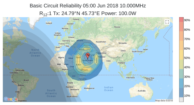
The Area page provides coverage predictions for a specified transmit site and traffic type.
The main page comprises a map display used to select the transmit site and display the prediction results, a toolbar to control display format and a series of panels to define prediction input parameters. Both single shot predictions and animations over a twenty-four hour period are supported.
The map toolbar is used to define the data to display on the map (Basic Circuit Reliability (BCR), Signal to Noise Ratio (SNR) or Signal Strength (S-Units)). The button activates the day/night overlay and the button is used to initiate the prediction. This button is enabled whenever the input panel settings becomes unsynchronised with the map overlay. A refresh indication is also displayed in the top right corner of the map whenever the map display does not correspond to the input values.
Alternatively, users may cycle through predictions for a twenty-four hour period by clicking the blue button in the toolbar under the map. The animation may be stopped by clicking the button. The step forward/backward buttons will increment/decrement the value of UTC and perform a prediction.
-
Specify the Transmit location. The Transmit location may be specified using one of the following methods;
-
Directly from the map by dragging the red 'Tx' map pin (
) to the required location. -
Using the Latitude / Longitude entry fields in the Tx. Site Panel.
-
Using the browser's geolocation support and clicking on the button (
) in the Tx. Site's entry panel. This will set the Tx. site to the user's current location (as reported by the browser).Privacy
Due to privacy concerns, most browsers only support geolocation services when securely connected to a site using https. Geolocation may not be supported when connecting to the site via http.
-
-
If required, toggle the button ON to reveal the raw ITURHFProp input/output text files which may be useful for debugging purposes. This data may be copied to the system clipboard by clicking the clipboard icon (
) in the Input File and Output File header bars. -
Select the plot resolution from “Low”, “Medium” and “High”, corresponding to sample points every 15°, 10° and 5° respectively.
High Resolution Predictions
Increasing resolution significantly increases processing time. Low resolution plots define 325 sample points (15° intervals), at High resolution (5° intervals) this increases to 2,701 data points.
-
Toggle the Day/Night display as required. This input has no effect on the prediction. The displayed day/night regions correspond to the time of the displayed prediction.
-
Specify the system parameters from the System panel;
- Date/Time
-
Specify the month/year for the prediction. The Date and Time datetimepickers are configured to only permit dates for which SSN values are available.
- Traffic
-
Specify the traffic type. This may be defined by selecting one of the predefined traffic types (derived from [ITU-R F.339-8] and [Lane 1997]) or user defined. Selecting 'User Defined' in the drop down menu will open a pair of text fields permitting the Bandwidth (0.005Hz - 3000000.0Hz) and required SNR (30.0dB and 200.0dB) parameters to be explicitly defined.
- Frequency
-
Specify the frequency (MHz) of the radiated signal in the range 2 < f < 30MHz.
- Power
-
Specify the net radiated power (W).
- Man-made Noise
-
Specifies the level of man-made noise at the receive location.
- SSN Source
-
[ITU-R P.371-8] states that SSN values used with P.533 are derived from the 'Standard Curves' published by WDC-SILSO, Royal Observatory of Belgium, Brussels. Users may wish to explore the use of other SSN data sets published the WDC-SILSO by making the appropriate selection from the drop-down list, refer to Section 10.1 for further information. If in doubt, the default 'Standard Curves' should be used.
-
Specify the Transmit antenna type using the Tx. Site entry panel.
-
If an isotropic antenna is specified, an antenna gain may also be defined. The default value of 2.16dBi corresponds to the gain of a dipole over an isotropic radiator
-
If a specific antenna type is selected, the bearing may also be defined.
-
-
Specify the Receive antenna gain using the Rx. Site Antenna Gain entry field. An isotropic antenna is assumed. The default value of 2.16dBi corresponds to the gain of a dipole over an isotropic radiator.
3.1. Displaying the Results
The predicted results are displayed directly onto the main map. The toolar below the map may be used to modify the presentation of the results;
- Colour
-
Selects the colormap used to represent the data from a drop-down menu containing a number of Plotly colour maps.
- Plot Type
-
Selects the plot type from a series of radio buttons, Basic Circuit Reliability (BCR), Signal to Noise Ratio (SNR) or Signal Strength (in S Units). Further information on S-Units may be found in Section 11, “S-Meter Values”.
- Day / Night
-
Toggles the Day / Night display, corresponding to the prediction UTC value.
- Download
-
Initiates a download of the map image, see Section 3.2 for further details.
3.2. Saving the Results
The button below the map is enabled whenever valid data is displayed. Clicking the button open a panel to select image parameters;
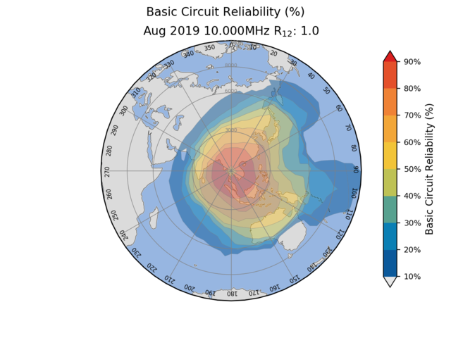
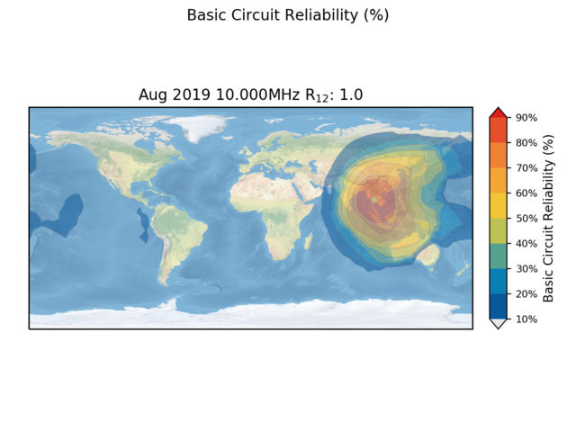
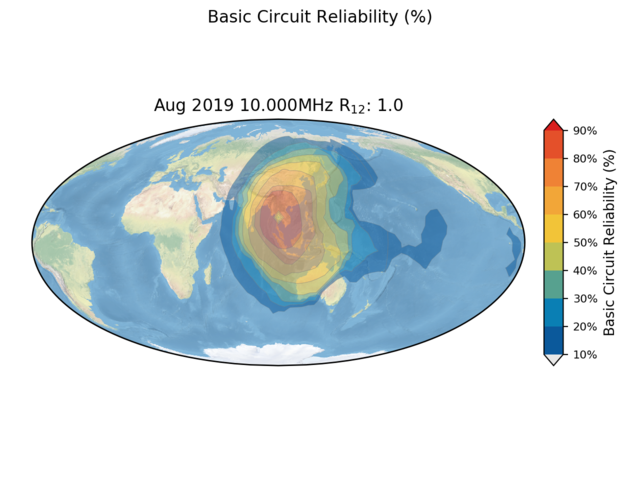
- Projection
-
Selects the map projection. Proppy currently supports Equidistant Cylindrical (Plate Carree), Azimuthal Equidistant and Mollweide projections. See Figures 1 to 3.
- Scale
-
A decimal value in the range 1.0 (smallest) to 4.0 (largest) that defines the map's scale. Applies to Azimuthal Equidistant projections only.
- LL Lat/Lng, UR Lat/Lng
-
Specifies the Latitude and Longitude of the Lower Left (LL) and Upper Right (UR) of the map. Applies to Equidistant Cylindrical (Plate Carree) projections only.
- Overlay
-
Specifies the map's appearance. Select from a graphical overlay, a basic mono display or a basic display with colours to identify land and oceans.
- Format
-
Select either .png or .pdf format. PNGs will be displayed in the browser window, PDFs will prompt a download.
The image may also be saved via the browser's print function. Media specific targets in the CSS file hide most of the page's content to reduce clutter, replacing the entry form with a title above the image.
4. Beacons
The 'Beacon' page displays the NCDXF/IARU International Beacon Project's scheduled transmissions and performs propagation predictions for the current month between each beacon and a specified receive site. For details of the project, please refer to the 'NCDXF/IARU website
The beacons page provides a real-time view of the beacon's transmissions, as shown in Figure 5.
4.1. Beacon's Propagation Prediction Method
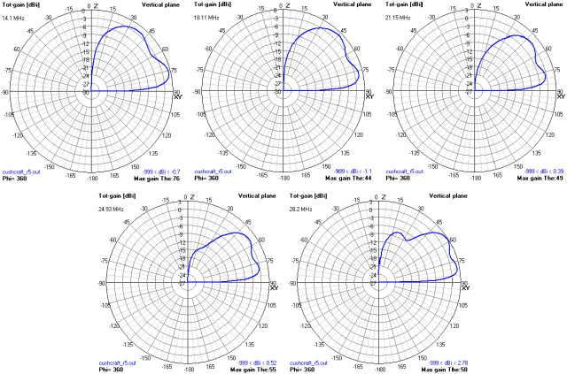
Each beacon comprises a 100W transmitter connected to a vertical (Cushcraft R5) antenna, operating at a forward power of 100W. The input file assumes a net radiated power of 90W (-10.46dBkW) to account for system losses.
Each beacon is assumed to be operating with a Cushcraft R5 antenna, employing a Type 14 antenna model.
-
Select the required SSN source. [ITU-R P.371-8] states that SSN values used with P.533 are derived from the 'Standard Curves' published by WDC-SILSO, Royal Observatory of Belgium, Brussels. Users may wish to explore the use of other SSN data sets published the WDC-SILSO by making the appropriate selection from the drop-down list, refer to Section 10.1 for further information. If in doubt, the default 'Standard Curves' should be used.
-
Specify the Receive location using one of the following methods;
-
Directly from the map by dragging the blue map pin (
) to the required location. -
Using the Latitude / Longitude entry fields in the Rx. Site Panel.
-
Using the browser's geolocation support and clicking on the button (
) in the Rx. Site's entry panel. This will set the Rx. site to the user's current location (as reported by the browser).
-
-
Specify the receive antenna gain. The Receive antenna type is assumed to be a isotropic radiator, with a user defined gain (dBi).
Receive Antenna Gain
The main user interface permits the gain of the receive antenna to be defined which may be used to tune the model as a whole, e.g. setting the receive antenna gain to -0.17dBi is equivalent to setting the antenna gain at each end of the link to zero (0dBi).
4.2. Saving the Results
Once prediction tables have been generated, they may be saved as a .pdf file in one of three formats;
-
A single page summary, using a format developed by Steve Nichols (G0KYA), containing S-Values for even numbered hours of the day (UTC). This table may be optionally be printed using colours to indicate predicted field strength.
-
A multipage document containing all predicted values. These tables may be optionally be printed using colours to indicate predicted field strength.
-
A multipage document containing all predicted values along with distances/bearings to each beacon from the receive site. These tables may be optionally be printed using colours to indicate predicted field strength.
4.3. Sample Input File
The following presents an input file describing the circuit between the beacon "YV5B" (Caracas, Venezuela) and a receive site in Cardiff, Wales. Eighteen similar runs, corresponding to the number of beacons, are produced to complete each prediction table.
PathName "Proppy Online HF Circuit Prediction: Beacon"
Path.L_tx.lat 9.083000
Path.L_tx.lng -67.833000
TXAntFilePath "path_to_data_directory/antennas/n14/o-cushcraft_r5.n14"
Path.L_rx.lat 51.482000
Path.L_rx.lng -3.179100
RXAntFilePath "ISOTROPIC"
RXGOS 2.16
Path.year 2018
Path.month  6
Path.hour 1,2,3,4,5,6,7,8,9,10,11,12,13,14,15,16,17,18,19,20,21,22,23,24
Path.SSN 1
Path.frequency 14.100, 18.110, 21.150, 24.930, 28.200
Path.txpower -10.46
Path.BW 500
Path.SNRr 0
Path.SNRXXp 90
Path.ManMadeNoise "RESIDENTIAL"
Path.Modulation "ANALOG"
Path.SorL "SHORTPATH"
RptFileFormat "RPT_PR"
DataFilePath "path_to_data_directory"
5. Planner Plots
The 'Planner' page allows a user to create propagation charts from a nominated transmit site to multiple receive sites on a single sheet, similar to those made available by the ARRL. The results are presented as a pdf download suitable for printing and retaining as a reference. All P2P plots on the chart are for a single Month/Year/SSN Value.
Processing Time
Planner charts are computationally expensive to create and take longer to process than individual P2P and Area plot types, up to 50 seconds for a full 12 chart plot.
All plots present the Operational MUF (OPMUF) upon which the 'Overlay' selector may be used to specify additional data representing either; Basic Circuit Reliability (BCR), Signal-to-Noise Ratio (SNR) or Signal Strength (S-Units).
After processing, the user is prompted with a dialogue box containing a link to download the completed prediction. Predictions may be saved in .pdf, .png or .svg formats.
On supported browsers, lists of receive sites may be saved in local storage for later recall. This allows users to set up a predefined list of specific sites of interest and return monthly to produce updated predictions.
-
Specify the Receive location(s). Up to 12 receive locations may be defined, although readability of the chart decreases with the number of receive locations. Receive locations are displayed on the map and in the corresponding table below the map. Each Receive Location is identified by a unique identity code and comprises a label (optional) and latitude and longitude. One receive location (id=0) is created when the page opens. Additional locations may either created manually using the button at the foot of the table or by importing a saved or preset lists. Once created, receive locations may be moved by either dragging on the map or direct entry in the appropriate latitude / longitude fields.
Receive site locations may also be retrieved from stored lists, either preset or user-defined saved lists;
- Preset Lists
-
Preset lists contain a set of predefined locations; 'Worldwide' and 'Europe' are currently supported, described in Section 5.1, “Presets”. Presets are selected using the drop down menu below the table and clicking on the button. Once loaded, receive site locations may be modified by either dragging the map markers or direct entry into the latitude / longitude fields.
- Saved Lists
-
On supported browsers, the contents of the table may be saved in 'localStorage' for later retrieval (the proppy website does not store any visitor data). On unsupported browsers, the / buttons are not displayed. The button is used to save the current contents of the table to the browser's localStorage. The is used to retrieve the saved set of receive sites.
-
Specify the plot parameters;
- Overlay
-
Defines the data overlay in the final plots.
- Colour
-
Defines the colour map used in the overlay (if defined).
- Format
-
Defines the file format for the plan.
-
Specify the system parameters from the System panel;
- Date
-
Specify the month / year for the prediction. These values, in conjunction with the nominated source of SSN values, will be used to determine the appropriate SSN for the prediction.
- Traffic
-
Specify the traffic type. This may be defined by selecting one of the predefined traffic types (derived from [ITU-R F.339-8] and [Lane 1997]) or user defined. Selecting 'User Defined' in the drop down menu will open a pair of text fields permitting the Bandwidth (0.005Hz - 3000000.0Hz) and required SNR (30.0dB and 200.0dB) parameters to be explicitly defined.
Note
This entry is only required if a data overlay is specified and is otherwise disabled.
- Power
-
Specify the net radiated power (W).
- Manmade Noise
-
Specifies the level of man-made noise at the receive location. This entry is only required if a data overlay is specified and is otherwise disabled.
- SSN Source
-
[ITU-R P.371-8] states that SSN values used with P.533 are derived from the 'Standard Curves' published by WDC-SILSO, Royal Observatory of Belgium, Brussels. Users may wish to explore the use of other SSN data sets published the WDC-SILSO by making the appropriate selection from the drop-down list, refer to Section 10.1 for further information. If in doubt, the default 'Standard Curves' should be used.
-
Specify the Transmit location using one of the following methods;
-
Directly from the map by dragging the red 'Tx' map pin (
) to the required location. -
Using the Latitude / Longitude entry fields in the Tx. Site Panel.
-
Using the browser's geolocation support and clicking on the button (
) in the Tx. Site's entry panel. This will set the Tx. site to the user's current location (as reported by the browser).Privacy
Due to privacy concerns, most browsers will require a secure (i.e. https) connection to the site. Geolocation may not be supported when connecting to the site via http.
A transmit site name may optionally be entered. This has no effect on the computation but if present will be used in the sub-plot title strings.
-
-
Specify the Transmit antenna gain using the Tx. Site Antenna Gain entry field. An isotropic antenna is assumed for p2p predictions. The default value of 2.16dBi corresponds to the gain of a dipole over an isotropic radiator.
-
Click the button to generate the predictions. Once complete, a link to the pdf document will be displayed in a modal box. The link will be valid for up to one hour from the plots being generated.
5.1. Presets
The following sections present the locations used in the preset values.
5.1.1. Worldwide
| ID | General Location | Actual Location | Latitude | Longitude |
|---|---|---|---|---|
| 0 | W. Europe | London, England | 51.5072 | -0.1275 |
| 1 | E. Europe | Kiev, Ukraine | 50.4500 | 30.5233 |
| 2 | East Coast | Washington, DC | 38.9047 | -77.0168 |
| 3 | Mid-USA | Kansas City, MO | 39.0997 | -94.5783 |
| 4 | West Coast | San Francisco, CA | 37.7833 | -122.4167 |
| 5 | Central Asia | New Delhi, India | 28.6139 | 77.2089 |
| 6 | Japan | Tokyo | 35.6833 | 139.6833 |
| 7 | Australia | Sydney | -33.865 | 151.2094 |
| 8 | Southern Africa | Lusaka, Zambia | -15.4167 | 28.2833 |
| 9 | South America | Asuncion, Paraguay | -25.3000 | -57.6333 |
| 10 | Hawaii | Honolulu | 21.3000 | -157.8167 |
| 11 | Caribbean | San Juan, Puerto Rico | 18.4064 | -66.0639 |
5.1.2. Europe
| ID | General Location | Actual Location | Latitude | Longitude |
|---|---|---|---|---|
| 0 | United Kingdom | London | 51.5072 | -0.1275 |
| 1 | Spain | Madrid | 40.3833 | -3.7167 |
| 2 | France | Paris | 48.8567 | 2.3508 |
| 3 | Finland | Helsinki | 60.16667 | 24.9333 |
| 4 | Ukraine | Kiev | 50.4500 | 30.5233 |
| 5 | Greece | Athens | 37.9840 | 23.7278 |
6. RadCom Predictions
The RadCom predictions page has been produced in collaboration with the RSGB's Propagation Studies Committee (PSC) and allows users to create tailored versions of RadCom's monthly propagation predictions, reflecting their preferred modes and equipment. Predictions are performed between a user's transmitter site and thirty-two globally distributed DX locations. The results indicate predicted power received (S-Units[1]) and Basic Circuit Reliability (%).
Transmit location is expressed as a Maidenhead Locator. If no transmitter position is defined, a default value corresponding to the centre of the United Kingdom is used. Locators may be provided in a four or six character format, the 4 character format typically being sufficient for HF circuits.
-
Specify the system parameters from the System panel;
- Date
-
Specify the month / year for the prediction. These values will be used to determine the appropriate SSN for the prediction.
- Traffic
-
Specify the traffic type. This may be defined by selecting one of the predefined traffic types (derived from [ITU-R F.339-8] and [Lane 1997]) or user defined. Selecting 'User Defined' in the drop down menu will open a pair of text fields permitting the Bandwidth (0.005Hz - 3000000.0Hz) and required SNR (30.0dB and 200.0dB) parameters to be explicitly defined.
- Power
-
Specify the net radiated power (W).
- Manmade Noise
-
Specifies the level of man-made noise at the receive location.
-
Specify the Transmit location using a Maidenhead Locator. The button at the right of the Locator entry field may be used to automatically determine the Locator using the browser's Geolocation API.
Privacy
The browser will request permission to access the user's location prior to accessing the Geolocation API. The conversion from latitude/longitude to Maidenhead Locator is performed locally at the client side and the latitude/longitude values of are not transmitted directly to the server.
-
Specify the Transmit and Receive antenna types using the Tx. Site/Rx. Site entry field. If an isotropic antenna is specified, a gain offset may also be specified. A value of 2.16dBi corresponds to the gain of a dipole over an isotropic radiator.
-
Click the button to start generating the predictions. Once complete, predictions may be saved as a pdf file for future reference by clicking the button at the bottom of the page.
6.1. Results
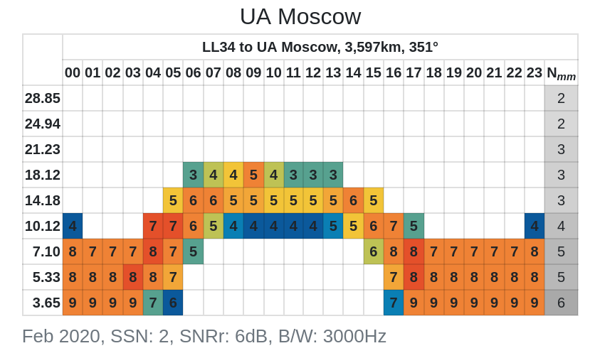
Figure 7 shows a table generated by the RadCom prediction, displaying predictions for each hour of the day (00:00-23:00) for each of the amateur bands. Cell content is defined by the Basic Circuit Reliability (BCR), receive signal strength (Pr), the 'Probability of Propagation' (PoP) and man-made noise.
In cases where BCR and PoP are both greater than 10%, the cell's background colour is used to indicate predicted reliability as indicated by the colour map at the top of the tables. In addition, the cell's content indicates Pr (expressed in S-Units). A bold font is used when Pr exceeds the predicted level of man-made noise, a normal font is used otherwise.
In the event that either BCR or PoP are less than 10%, the cell is left blank. Actual values for BCR, PoP and Pr may be seen by hovering above the cell.
6.2. Sample Input File
The following presents a typical input when performing a RadCom prediction. The sample shown is for a circuit passing CW traffic between the UK and Moscow (55.7558, 37.6173). Thirty-two similar runs are performed to complete each set of predictions.
Path.L_tx.lat 52.000000
Path.L_tx.lng -2.000000
TXAntFilePath "/path_to_antenna_files/d10m.n14"
Path.L_rx.lat 55.755800
Path.L_rx.lng 37.617300
RXAntFilePath "/path_to_antenna_files/d10m.n14"
Path.year 2019
Path.month 2
Path.hour 1, 2, 3, 4, 5, 6, 7, 8, 9, 10, 11, 12, 13, 14, 15, 16, 17, 18, 19, 20, 21, 22, 23, 24
Path.SSN 3
Path.frequency 28.85, 24.94, 21.225, 18.118, 14.175, 10.125, 7.1, 5.33, 3.65
Path.txpower -10.00
Path.BW 500.00
Path.SNRr 0.00
Path.SNRXXp 90
Path.ManMadeNoise "RURAL"
Path.SorL "SHORTPATH"
RptFileFormat "RPT_BCR | RPT_PR"
LL.lat 55.755800
LL.lng 37.617300
LR.lat 55.755800
LR.lng 37.617300
UL.lat 55.755800
UL.lng 37.617300
UR.lat 55.755800
UR.lng 37.617300
DataFilePath "path_to_data_directory"
7. Shortwave Listening Schedules
The 'SWL' page may be used to interrogate the current HFCC database of scheduled shortwave transmissions to access programming of interest. The underlying database is made freely available by the HFCC at http://www.hfcc.org/data/.
The main page comprises a map, used for defining the target location, and a 'Search Filters' panel incorporating filters for frequency, time, language and target CIRAF zones. Filters are enabled/disabled using the checkbox at the right-hand side of each entry field.
- Frequency
-
Filtering by frequency selection may be achieved by either entering a value directly into the frequency text field or selecting a band using the band entry field. The search may be expanded by ±5kHz by clicking the horizontal arrow (↔) button in the right of the text entry field; i.e. if the specified frequency is '6.195', clicking the ↔ button will return results for the range 6.190-7.200MHz.
The frequency and band entry fields are mutually exclusive; activating one will disable the other if it is already enabled.
- Language
-
Clicking the checkbox in the left of the text field will filter the results to include only the language specified in the language drop-down box.
- Time
-
Clicking the checkbox in the left of the text field will filter the results to include only stations active at the specified time (UTC).
The 'clock' push-button may be used to set the time to any required value.
The 'play' button will synchronise the time with the computer's clock. The position of the day/night overlay on the map corresponds to the value in the time field.
- CIRAF
-
Clicking the checkbox in the left of the text field will filter the results to include only those directed to the CIRAF zones specified. See https://www.itu.int/net/ITU-R/terrestrial/broadcast/hf/refdata/maps/index.html for details of the CIRAF zones. Clicking the (
 ) at the right of the CIRAF entry field will replace the contents of the field with the CIRAF zone corresponding to the latitude/longitude values at the top of the page. Clicking on the button (
 ) button will select the CIRAF zone currently specified along with all adjacent zones. If no zone is specified, the zone corresponding to the latitude/longitude values at the top of the page is used.
Example:
'39'specifies a single zone.'18,19, 27-29'will filter results to transmissions targeting CIRAF zones 18, 19, 27, 28 & 29 (corresponding to most of Western Europe).
The button is used to initiate the search, displaying the results in a table below the filter panel. The table includes a search facility to further refine the results along with the ability to re-order the results by clicking on the table headers.
Results may be saved to file in either CSV (suitable for importing into Excel) or as a pdf document by selecting the required format at the bottom of the table and clicking the button.
The sites displayed in the table are also indicated on the map as shown in Figure 8 below;
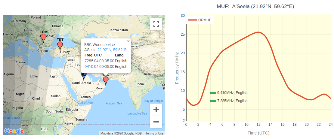
Clicking on any of the sites in the main map will open a small information window providing additional data and initiate a propagation prediction between the transmitter site and the user received site. Clicking on the sites coordinates in the information window will open a new tab displaying the site's location on Google Maps. Note: Many of the site locations are taken from the site.txt file distributed with the HFCC schedules and are not necessarily precise enough to show the exact location of the site.
7.1. URL Parameters
The URL is updated to include the input parameters when the results are updated. This URL may be copied and shared with other users in social media groups etc.
7.2. CIRAF Zones
CIRAF zones (`Conferencia Internacional de Radiodifusión por Altas Frecuencias') are used by the ITU to identify target coverage areas as shown in Figure 9 below;
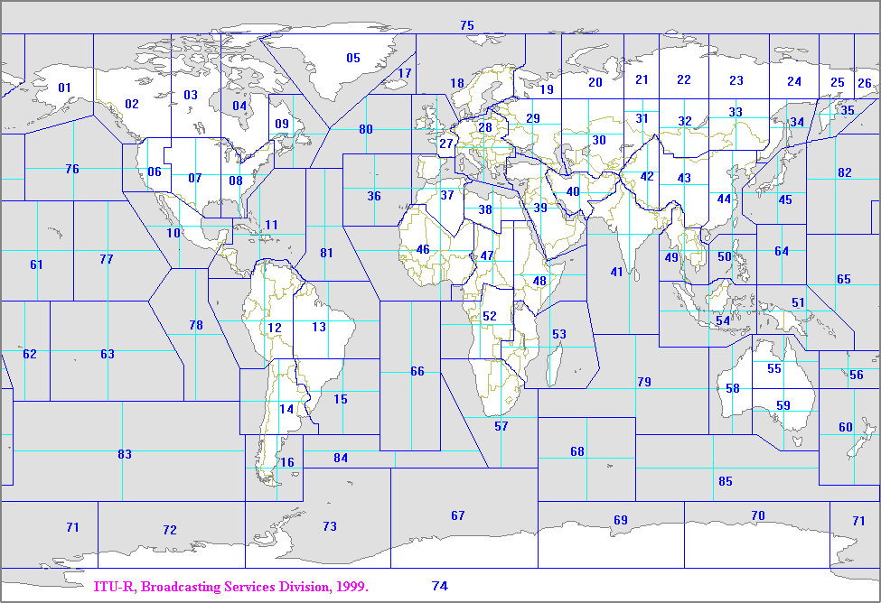
Proppy determines the CIRAF zone by comparing the entered lat/lng values with 911 CIRAF test points defined by the ITU (https://www.itu.int/en/ITU-R/terrestrial/broadcast/HFBC/Pages/Reference.aspx).
7.3. Example Searches
Figure 10 shows a search configured to show all stations active at 10:42UTC on frequencies between 6.190-6.200 (e.g. 6.195MHz±5kHz).
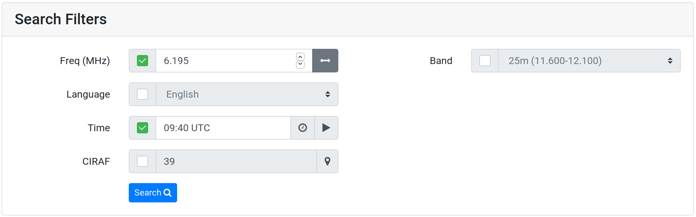
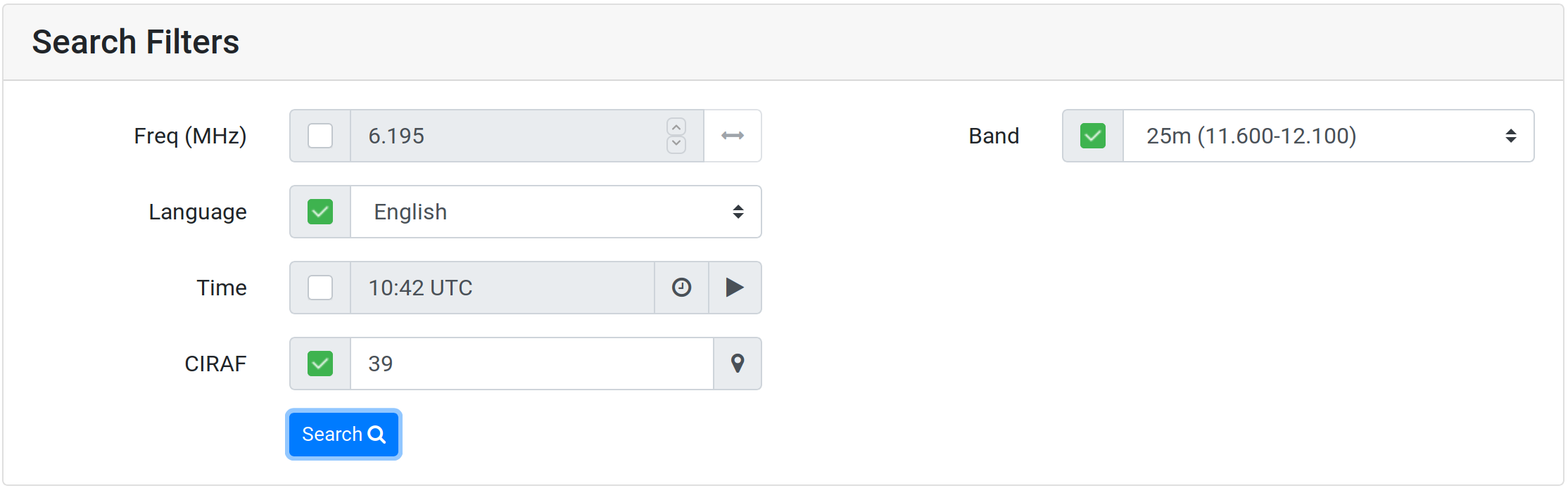
Figure 11 shows a search configured to show all English language transmissions in the 25m band (11.600-12.100MHz) directed to CIRAF Zone 39 (Middle East).
8. Web Service
Proppy may also be used as a web services, allowing HTML 'GET' parameters to be used to create images on demand. Only area and planner type plots are currently supported, point-to-point plots are a planned enhancement. The area web service is available at the following URL, to which correctly formatted parameters shall be be appended.
https://soundbytes.asia/proppy/ws/areaA minimal example of a correctly formatted request is;
https://soundbytes.asia/proppy/ws/area?tx=23.1,-82.3&freq=10.26
Plots returned by the web service are in the Portable Network Graphics (PNG) format and may be saved in a browser or indeed called up as part of an image element in a web page.
8.1. Area
The Area Web Service returns area prediction plots in response to HTML requests. Input variable are defined in the URL e.g; The following request parameters were used to create the plot shown in Figure 12;
pwr=100&tx=23.1,-82.3&freq=10.26&ll=-50,-120.45&ur=50,0
The web service accepts the parameters listed below. When multiple parameters are used, the '&' character shall be used as a separator.
Encoding
The '&' symbol is a reserved character and requires encoding prior to sending to the server. Most browsers will perform the required encoding automatically when entering the URL in the address bar. However, client applications may need to explicitly encode the parameter string, . e.g. Python 3 uses the urllib.parse.quote() function to replace ampersand symbols with the corresponding 'percent encoded' equivalent ('%26').
- tx
-
Required. A pair (lat, lng) of float values specifying the coordinates of the transmitter location. Positive values should be used to express North and East directions. Negative values should be used to express South and West.
Example: '
tx=54.23,2.4' specifies a transmitter located at 54.23°N, 2.4°E. - freq
-
Required. Float value [2.0-30.0] specifying the frequency of operation in MHz.
Example: '
freq=10.265' specifies a frequency of 10.265MHz. - pwr
-
Optional. Integer value [1-1000000000] specifying the transmitter power in Watts. Defaults to 100W if not specified.
Example: '
pwr=1000' sets the transmitter power to 1000W / 1kW. - bw
-
Optional. Float value [0.005-3000000.0] specifying the bandwidth of the traffic. See Section 12 for examples of recommended bandwidths. Defaults to 3000 if not specified.
Example: '
bw=500' sets the bandwidth to 500. - snr
-
Optional. Float value [30.0-200.0] specifying the snr required to support the traffic type. See Section 12 for examples of recommended SNR values. Defaults to 15 if not specified.
Example: '
snr=500' sets the required SNR to 500. - ssn
-
Optional. Integer value [1-311] specifying the ssn value to be used in the calculations. If no value for ssn is provided, the y and m parameters will be used to define the value from the SIDC Standard Curves dataset.
Example: '
ssn=6' sets the ssn to 6. - y
-
Optional. Integer value specifying the year for the prediction. Default value: Current year.
The month ('m') and year ('y') parameters are used to define the month for the prediction. If no value for ssn is provided, the m,y parameters will be used to retrieve the correct value of SSN. If ssn is provided, the y value will be used as a label only and have no influence on the calculations. Valid values define a month/year for which SSN values are available. The is generally the period January 2005 through to eleven months from the current date. Valid values are shown in the tables on SSN Data Page.
Example: '
y=2017' sets the year to 2017. - m
-
Optional. Integer value [1-12] specifying the month for the prediction. Default value: Current month.
Example: '
m=3' sets the month to March. - utc
-
Optional. Integer value [1-24] specifying the hour (UTC) for the prediction. Default value: Current time (UTC).
Example: '
utc=7' sets the time (UTC) to 07:00. - ll
-
Optional. A pair (lat, lng) of float values specifying the coordinates of the lower left corner of the plot. Positive values should be used to express North and East directions. Negative values should be used to express South and West. Default:-90,-180 (180°W, 90°S)
Example: '
ll=10.25,-120' places the lower left of the plot at 10.25°N, 120°W. - ur
-
Optional. A pair (lat, lng) of float values specifying the coordinates of the upper right corner of the final plot. Positive values should be used to express North and East directions. Negative values should be used to express South and West. Default:90,180 (180°E, 90°N).
Example: '
ur=50,-60.1' places the upper right of the plot at 10°N, 60.1°W. - ptype
-
Optional. String value from the set ('bcr', 'snr', 'e'), representing Basic Circuit Reliability, Signal to Noise Ratio and Field Strength respectively. Default: bcr
Example: '
type=snr' specifies the display of Signal to Noise data.
8.2. Planner
The Planner Web Service returns area prediction plots in response to HTML requests. Input variable are defined in the URL e.g; The following request parameters were used to create the plot shown in Figure 13;
https://soundbytes.asia/proppy/ws/planner?qth=QTH,24.69,46.76
&site=Nakorn%20Sawan,15.81,100.06&site=London,51.507,-0.128
&site=Jakarta,-6.22,106.88&site=Negombo,7.23,79.84
&bw=500&snr=0&ptype=bcr&pwr=5&ftype=png&tz=3

The web service accepts the parameters listed below. When multiple parameters are used, the '&' character shall be used as a separator.
Encoding
The '&' symbol is a reserved character and requires encoding prior to sending to the server. Most browsers will perform the required encoding automatically when entering the URL in the address bar. However, client applications may need to explicitly encode the parameter string. e.g. Python 3 uses the urllib.parse.quote() function to replace ampersand symbols with the corresponding 'percent encoded' equivalent ('%26').
- qth
-
site=name,lat,lng Required
Comprises three elements specifying the name, latitude and longitude of the operator's location.
name A character string representing the name of the operator's location which will be used in the plot titles. Spaces are permitted but the use of the reserved characters (?#,&) is not supported and will generate an error. For future compatibility, it is recommended that none of the reserved characters defined in RFC3986 are used.
lat a float values specifying the latitude of the of the transmitter home location. Positive values should be used to express North, negative values should be used to express South.
lng a float values specifying the longitude of the of the transmitter home location. Positive values should be used to express East, negative values should be used to express West.
Example: '
qth=London,51.507,-0.128',qth=Chiang Mai,18.795,98.999 - site
-
site=name,lat,lng Required (at least once)
site=name,lat,lng,sorl
Comprises three elements specifying the name, latitude and longitude of the target locations. An optional parameter, sorl may be used to specify if a short or long path should be used in the prdiction. Up to twelve sites may be specified.
name A character string representing the name of the target location which will be used in the plot titles. Spaces are permitted but the use of the reserved characters (?#,&) is not supported and will generate an error. For future compatibility, it is recommended that none of the reserved characters defined in RFC3986 are used.
lat a float values specifying the latitude of the of the target location. Positive values should be used to express North, negative values should be used to express South.
lng a float values specifying the longitude of the of the target location. Positive values should be used to express East, negative values should be used to express West.
sorl (Optional) a single character ('S' or 'L') values specifying if the long or short path should be used. This is an optional parameter, if not defined the short path is assumed.
Example: '
site=London,51.507,-0.128,L&site=Riyadh,24.633,46.717' specifies two sites, using the long path to the first site. - ptype
-
ptype=bcr|pr|snr Optional. Default = OPMUF (no overlay)
The parameter is used to define the optional data overlay.
Example: '
ptype=snr' - month
-
month=[1-12] Optional: Default = current month
An integer representing the month of the year (January = 1, December = 12).
Example: '
month=6' - year
-
year=[2005-2025] Optional. Default = current year.
An integer representing the year. Default is the current year.
Example: '
year=2024' - tz
-
tz=[-12-12] Optional. Default = 0
Defines the timezone to be used on the time axis, allowing the results to be displayed in the the user's local timezone. Timezones East of Greenwich shall be expressed as positive values, West of Greenwich shall be expresses as negative values.
Example: '
tz=7' specifies a time zone GMT+7 (Bangkok, Thailand). 'tz=-4' specifies a time zone GMT-4 (New York, USA). - cmap
-
cmap=jet|gnuplot|gnuplot2|voacap Optional. Default = 'jet'
Defines the colourmap used when generating the plot.
Example: '
cmap=gnuplot' - pwr
-
pwr=[1-1000000000] Optional. Default = 100
The transmit power in Watts.
Example: '
pwr=150' specifies a tranmit power os 150W. - bw
-
bw=[30.0-24000.0] Optional. Default = 3000
Audio bandwidth. Refer to Section 12 for details of bandwidths/SNRs required to support traffic types.
Example: '
bw=500' (500Hz) - snr
-
snr=[-50.0-60.0] Optional. Default = 15
Required SNR in dB. Refer to Section 12 for details of bandwidths/SNRs required to support traffic types.
Example: '
txgain=6' - noise
-
noise=city|residential|rural|quietrural|quiet|noisy Optional. Default = rural
Defines the man made noise level at the remote receive site.
Example: '
noise=residential' - txgain
-
txgain=(float) Optional. Default = 2.16
Gain of the trasmitter antenna, dB relative to an isotrpic radiator.
Example: '
txgain=3.2' - ftype
-
ftype=pdf|png|svg Optional. Default = pdf
Specify the file type.
Example: '
ftype=png'
9. Spaceweather
The spaceweather page presents data extracted from the latest Geophiysical Alert Message published by NOAA at http://services.swpc.noaa.gov/text/wwv.txt. Updates to this data are typically published at three hourly intervals from around 00:00UTC.
:Product: Geophysical Alert Message wwv.txt
:Issued: 2017 Sep 09 0910 UTC
# Prepared by the US Dept. of Commerce, NOAA, Space Weather Prediction Center
#
# Geophysical Alert Message
#
Solar-terrestrial indices for 08 September follow.
Solar flux 117 and estimated planetary A-index 96.
The estimated planetary K-index at 0900 UTC on 09 September was 2.
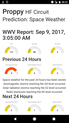
Space weather for the past 24 hours has been severe.
Geomagnetic storms reaching the G4 level occurred.
Solar radiation storms reaching the S1 level occurred.
Radio blackouts reaching the R1 level occurred.
Space weather for the next 24 hours is predicted to be moderate.
Geomagnetic storms reaching the G1 level are expected.
Solar radiation storms reaching the S1 level are expected.
Radio blackouts reaching the R2 level are expected.Reports are retrieved every three hours and parsed to extract the data to drive a graphical display, as shown in the following screenshot.
10. Sun Spot Numbers (SSNs)
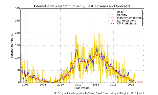
Determination of ionospheric characteristics related to HF propagation requires knowledge of the prevailing levels of solar activity [ITU-R P.1239-3]. The Sunspot Number (SSN), quantifying of the number of dark spots visible on the Sun’s surface, has historically served as the primary proxy of solar activity [Clette et al. 2015]. Records of SSNs date back over 400 years, providing a valuable insight into the sun's quasi periodic 11-year cycle of activity. Superimposed onto this cycle are shorter term variations that can result in large fluctuations in day-to-day values. More recent research suggests that the 11 year cycle is itself modulated by the interaction of two solar dynamos, accounting for the fluctuations in the level of activity observed during each cycle [Zharkova et al., 2015].
The figure below illustrates how daily values (yellow) may be averaged over month (blue) and monthly smoothed (12-month) (red) periods, eliminating complex short term variations to yield a more predictable indicator of solar activity. The preferred ionospheric metric when determining the critical frequencies of the various layers and the MUF factor M(3000)F2 is a 12-month running mean sunspot number, R12 [ITU-R P.1239-3]. R12 values are a function of sunspot values extending at least six months either side of the month of interest [ITU-R P.371-8]. (Note that this has the unfortunate side effect that an R12 value for a given month “m” cannot be absolutely determined until “m+6” (six months later)).
10.1. SSN Data
In accordance with Recommendation [ITU-R P.371-8] Proppy uses SSN (R12) values presented in the ITU's Circular of Basic Indices for Ionospheric Propagation, derived from 'Standard Curves' dataset provided by WDC-SILSO, Royal Observatory of Belgium, Brussels.
In addition to the Standard Curves (SC) dataset, the SIDC publish predictions based on the Combined Model (CM) and the McNish & Lincoln (M&L) method.
- Standard Curves
-
Based on the sunspot number with and uses mean-cycle curves derived from historical data to produce predictions. The Standard curves are considered to be effective at predicting the declining phase of a cycle but breaks down when approaching the minima so is not so reliable at predicting the rise of the successive cycle.
- Combined Method
-
The combined method makes predictions based on the sunspot number, comparing all cycles recorded since 1749, combined with an assessment using the the geomagnetic index (aa). The geomagnetic index, 'aa', is an indicator of the level of future solar activity. For this reason, the Combined Model may produce superior results when passing the Solar minimum.
- McNish & Lincoln
-
The McNish & Lincoln method is the most established of the three models, dating back to 1949, and is of interest for largely historical reasons. As with the Standard Curves method, only the sunspot is considered as an input which in this case is compared to historical data for the period 1849 to 1975 (cycles 9 to 20). This provides fair predictive abilities for much of the cycle but, in common with the Standard Curves method, is less effective at the minima (±1.5 year).
Users may therefore wish to experiment with the Combined Model (both with and without the Kalman Filter) in a bid to improve prediction accuracy.
The SSN values used by Proppy are presented at https://soundbytes.asia/proppy/help/ssn. These values extend from 2005 to the latest available prediction date (typically 12 months ahead).
11. S-Meter Values
S-Meter values are commonly used to express received signal strength. Proppy derives S-Meter values from the median available receiver power (Pr dBW) predicted by ITURHFProp[2]. This value represents the summation of the the powers arising from the different modes, each mode contribution depending on the receiving antenna gain in the direction of incidence of that mode. The median received power levels are converted to S-Meter readings for ease of intelligibility. The conversion to S-Values follows the IARU Region 1 Technical Recommendation R.1, S9 for the HF bands to be a receiver input power of -103 dBW.
| S-Meter | dB(1uV/m) | dBW | Subjective Assessment |
|---|---|---|---|
| S9 | 33.98 | -103 | Very strong signals |
| S8 | 27.96 | -109 | Strong |
| S7 | 21.94 | -115 | Moderately strong |
| S6 | 15.92 | -121 | Good |
| S5 | 9.90 | -127 | Fairly good |
| S4 | 3.88 | -133 | Fair |
| S3 | -2.14 | -139 | Weak |
| S2 | -8.16 | -145 | Very weak |
| S1 | -14.19 | -151 | Faint signal, barely perceptible |
12. Traffic Types
Proppy uses values of SNR and bandwidth derived from [ITU-R F.339-8] and [Lane 1997] as follows;
| Traffic | SNR (dB) | Bandwidth (Hz) |
|---|---|---|
| CW | 0 | 500 |
| SSB (Usable) | 6 | 3000 |
| SSB (Marginal) | 15 | 3000 |
| SSB (Commercial) | 33 | 3000 |
| SWBC (Fair) | 36 | 5000 |
| SWBC (Good) | 48 | 5000 |
13. Troubleshooting
13.1. Cache
The site is under constant development and it is possible that cached resources conflict with newer resources on the site. Many problems can therefore be resolved by simply reloading a fresh copy of the page. The procedure for this varies by browser / platform but often based around the Ctrl-F5 key combination. Further information on this process may be found at https://en.wikipedia.org/wiki/Wikipedia:Bypass_your_cache#Bypassing_cache.13.2. Validation Error: [csrf_token] The CSRF token has expired.
The site is protected against Cross-site request forgery (CSRF), also known as one-click attack or session riding, a type of malicious exploit of a website where unauthorized commands are transmitted from a user that the website trusts. This requires a token to be issued to the client browser for each session. If this token expires, data submitted by the client will fail to validate.
If this error message is seen, simply reload the page.
13.3. Geo Location Error
In order to protect user's privacy, most current browsers prevent the transmission of personal data over unsecured channels. If this error message is seen, reconnect to the website using the https protocol, e.g. https://soundbytes.asia/proppy/.
13.4. Supported browsers
The site is built using the Bootstrap 4 Framework, supported by the latest stabe releases of all major browsers and platforms. On Windows, Internet Explorer 10-11 / Microsoft Edge are supported - IE9 and down is not.
Full details of browser and device support may be found at https://getbootstrap.com/docs/4.0/getting-started/browsers-devices/"
14. Privacy
14.1. Cookies
The website uses “cookies”, to retain user preferences between visits. These are stored on the user's machine so that subsequent page loads are initialised with the user's preferences and language. The values of the cookie are not stored by the server nor distributed to any third party.
The cookies ('locale', 'txlat', 'txlng', 'rxlat', 'rxlng') are not encrypted and may be readily examined using a browser's cookie manager. These cookies are designed to persist between sessions for up to six months but may be deleted by the user at any time.
- txlat, txlng
-
Coordinates of the preferred Transmit location.
- rxlat, rxlng
-
Coordinates of the preferred Receive location.
- traffic
-
A string representing the preferred traffic type, used to set the Traffic drop down menus when a page is opened.
- mute-wwv-msg
-
This cookie is set when a user closes a WWV warning message and is used to suppress further messages for three hours (the interval at which WWV warnings are published).
- locale
-
Used by the site to store an ISO code identifiying a user's preferred language (e.g. 'de', 'es' etc.). Users who only use English may not see this cookie.
In addition to the above cookies which are used directly by the Proppy application, the following cookies are associated with the site.
- session
-
Created by the Flask Framework used to build the site and is used to store the variables '_id' and the 'csrf_token'. This is a HTTP Only cookie and inaccessible to the Javascript. Proppy does not store any values in this cookie.
14.2. HTTPS
It is recommended that users access the site using the secure https protocol; https://soundbytes.asia/proppy.
15. Language Preferences
Proppy's calculation pages are offered in the following languages;
-
Arabic (ar)
-
English (en-gb)
-
Finnish (fi)
-
French (fr)
-
German (de)
-
Spanish (es)
Language selection is made via the menu presented at the foot of each page. This will set a cookie ('locale') to preserve the user's language preference between visits.
In the event that a 'locale' cookie is not found, the value of the request header's 'Accept-Language' parameter is used to identify the required language.
Glossary
- Basic Circuit Reliability
-
The probability that the specified performance criterion (i.e. the specified signal-to-noise) is achieved. For analogue systems, it is evaluated on the basis of signal-to-noise ratios incorporating within-an-hour and day-to-day decile variations of both signal field strength and noise background. [ITU-R P.842-5]
- Basic MUF
-
The highest frequency by which a radio-wave can propagate between given terminals, on a specified occasion, by ionospheric refraction alone [ITU-R P.373-9]
- Maidenhead Locator
-
The Maidenhead Locator System is a geographic co-ordinate system used by amateur radio operators to succinctly describe their locations. A locator comprises alternating pairs of letters and digits to define a Field/Square/Subsquare.
- Operational MUF
-
The highest frequency that would permit acceptable performance of a radio circuit by signal propagation via the ionosphere between given terminals at a given time under specified working conditions. OPMUF is derived from the BMUF by the application of a correction factor (in the range 1.10--1.35) [ITU-R P.373-9]
Bibliography
[Clette et al. 2015] 2015. The Solar Activity Cycle. 35-103. Revisiting the sunspot number. https://arxiv.org/pdf/1407.3231.pdf.
[ITU-R P.533] Recommendation P.533-14. August 2019. International Telecommunication Union. Method for the prediction of the performance of HF circuits. https://www.itu.int/rec/R-REC-P.533-14-201908-I/en.
[ITU-R F.339-8] Recommendation F.339-8. February 2013. International Telecommunication Union. Bandwidths, Signal-to-Noise Ratios and Fading Allowances in HF Fixed and Land Mobile Radiocommunication Systems. https://www.itu.int/rec/R-REC-F.339/en.
[ITU-R P.373-9] Recommendation P.373-9. September 2013. International Telecommunication Union. Definitions of maximum and minimum transmission frequencies. https://www.itu.int/rec/R-REC-P.373/en.
[ITU-R P.842-5] Recommendation P.842-5. August 2013. International Telecommunication Union. Computation of reliability and compatibility of HF radio systems. https://www.itu.int/rec/R-REC-P.842/en.
[ITU-R P.1239-3] Recommendation P.1239-3. February 2012. International Telecommunication Union. ITU-R reference ionospheric characteristics. https://www.itu.int/rec/R-REC-P.1239/en.
[ITU-R 1240-2] Recommendation P.1240-2. September 2013. International Telecommunication Union. ITU-R methods of basic MUF, operational MUF and ray-path prediction. https://www.itu.int/rec/R-REC-P.1240-2-201507-I/en.
[Lane 1997] 1997. Radio Science. 2091-2098. Required Signal-to-Interference Ratios for Shortwave Broadcasting. http://onlinelibrary.wiley.com/doi/10.1029/97RS00843/pdf.
[Lane 2005] 2005. Ionospheric Effects Symposium, Alexandria VA USA. Improved guidelines for automatic link establishment operations.. http://www.voacap.com/documents/GLane_ALE.pdf.
[Zharkova et al., 2015] 2015. Scientific reports. Heartbeat of the Sun from Principal Component Analysis and prediction of solar activity on a millennium timescale. https://www.ncbi.nlm.nih.gov/pmc/articles/PMC4625153/.
[1] Refer to Section 11, “S-Meter Values” for a description of S-Units.
[2] See Rec. ITU-R P.533-14, Section 6, Median available receiver power